The Convolutional Neural Network

I. Introduction
The last few posts I’ve written about AI consciousness and infinite suffering have been fairly dire, so I decided to switch things up and write about something more practical: the convolutional neural network. While working on a research proposal about circuit stability during fine-tuning, I spent a few hours talking with Grok about what CNNs actually are. What I eventually realized is that CNNs, while conceptually different from typical feed-forward neural networks, are surprisingly intuitive and powerful in practice. This post breaks down what convolutional neural networks are in simple terms. In a later post, I’ll walk through experiments that show just how efficient they can be.
II. Feed-Forward, Artificial Neural Networks
I'm assuming most people reading this already have some introductory knowledge about traditional, feed-forward, artificial neural networks. That's certainly where I came from, so I can explain it best from that perspective. However, to ensure everyone is on the same page, I've included a brief recap of ANNs.
The artificial neural network gave way to deep learning, a field focused on training multi-layered networks to learn hierarchical representations of data. Before neural networks, machine learning consisted largely of simpler statistical methods: linear regressions, decision trees, SVMs, and basic pattern matching algorithms like TF-IDF for text processing. Neural networks were novel not only because they brought us closer to modeling the human brain, but also because of the 'universal approximation theorem,' which showed that neural networks with a single hidden layer, enough neurons, and non-linear activation functions could approximate any continuous function (Cybenko, 1989). Of course, approximating any continuous function would require a network of impractically large size. However, even small neural networks can complete fairly complex tasks.
With that, we can begin a more technical explanation of how ANNs work. This might feel dense at first, so feel free to skim and rely on the visual depictions instead.
At a high level, a neural network is made up of layers of neurons. Each neuron in a layer connects to every neuron in the layers before and after it, creating a dense web of connections. Each connection between neurons is called a ‘weight’ or ‘edge,’ while the neurons themselves are called ‘nodes.’
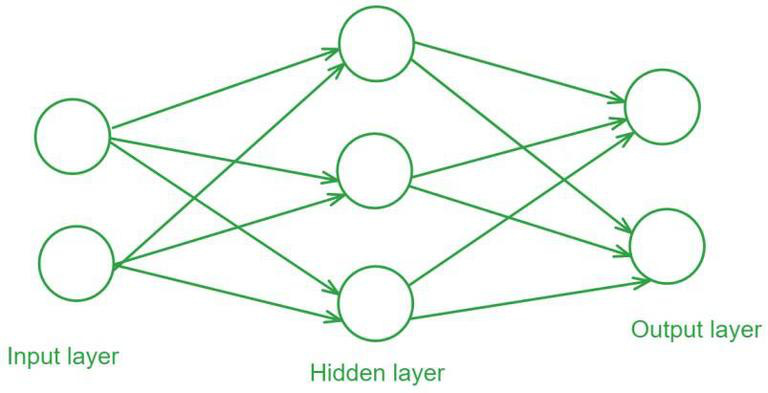
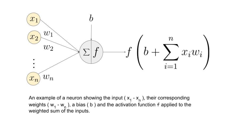
Networks start with an 'input layer' and end with an 'output layer.' Each neuron in the input layer takes in a number and passes it forward. Each connection takes its neuron's value, multiplies it by a 'weight,' and adds a constant called a 'bias.' Since multiple neurons feed into each neuron in the next layer, the receiving neuron adds up all these weighted and biased values.
This process repeats layer by layer until you reach the output. A slightly different process occurs in hidden-layer neurons (neurons in between the input and output layers). After computing their sums, each hidden-layer neuron applies an ‘activation function’ (like sigmoid, ReLU, or tanh). These functions introduce non-linearity into the network, which allows networks to solve nonlinear problems, since stacking linear operations on top of each other still gives you a linear operation. After applying the activation function, the result gets weighted and biased again before moving to the next layer.
During training, only the weights and biases change through a process called backpropagation. That’s beyond the scope of this post, but this video by 3Blue1Brown and this article by AWS Machine Learning University explain it well for anyone interested.
Forward propagation, for the most part, consists of linear algebra and matrix multiplications: This link has a comprehensive guide to the underlying math.
III. The Convolution
Given the power of ANNs, it might seem counterintuitive that we’d need an entirely new type of neural network for the relatively simple task of image classification. If we try to use traditional ANNs for this, we’d need to flatten the image into a vector of pixel values. This creates three major problems:
Loss of Spatial Information: Each neuron only sees its own value and can't access what neighboring neurons contain. This means relationships between nearby pixels are nearly impossible to capture in traditional neural networks, since each neuron's value is unaffected by surrounding pixels. This is problematic because a single pixel only makes sense in the context of its neighbors. A black pixel might be part of an eye OR meaningless noise depending on what’s around it.
Parameter Counts: Consider an image with dimensions h × w. For simplicity, assume it's black and white, so each pixel is either 1 (white) or 0 (black). Since each input neuron handles one pixel, you'd need h × w neurons in the input layer. That means h × w weights and biases just for the connections between the input layer and the first hidden layer before accounting for all the subsequent layers. A modest 224 × 224 pixel image would require 50,176 parameters just for the first layer, making training slow and memory-intensive.
Fixed Input Sizes: Since each neuron corresponds to one pixel and the neuron count is fixed during training, you can only use images of a predetermined size. If you initialize 784 input neurons (for a 28 × 28 image), you can't feed in images of any other dimension without completely retraining the network.
Convolutional neural networks solve these problems.
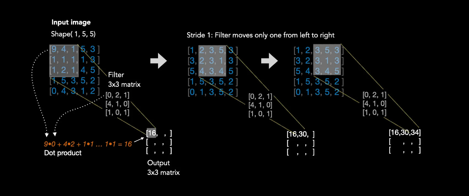
We’ll start with the most fundamental part of a CNN: the ‘kernel.’ A kernel is a small square grid of weights that slides over an image like a filter. Let’s consider a 3×3 kernel, meaning it has 9 weights arranged in a 3×3 grid. Now imagine a simple 28×28 black-and-white image where each pixel is either 0 (black) or 1 (white).
Here’s how it works: you place the 3×3 kernel over the top-left corner of the image. Each of the 9 weights in the kernel overlaps with one pixel. You multiply each kernel weight by its corresponding pixel value, then add all 9 products together. This sum becomes a single number representing that 3×3 patch of the image.
This multiplication is called the Hadamard product (element-wise multiplication), written as A ⊙ B. For example:
The kernel’s values are the ‘weights,’ and the image’s pixel values are the 1s and 0s. Then, the network will sum together all of the weighted pixel values and place that value in the center of the kernel. Given our above matrix, the sum of all elements is 1 + (-1) + 1 + (-1) = 0.
Now the kernel has processed 9 pixels. To capture the rest of the image, the kernel slides over by a specified number of pixels (typically 1) and repeats the process. This sliding distance is called the ‘stride.’
After sliding across the entire image, you end up with a new matrix of these summed values. This output is slightly smaller than the original image because the kernel can’t fully cover the edges. For instance, a 3×3 kernel with stride 1 applied to a 28×28 image produces a 26×26 output matrix.
This might feel abstract, so here’s an analogy: imagine you’re a detective analyzing photos to find knives at crime scenes. You use a magnifying glass that shows you a 3×3 inch area at a time. You slide it across the photo, moving 1 inch over after each look. At each position, you check whether the features in that small area match what a knife looks like. The kernel works the same way. It’s looking for specific patterns (like edges or shapes) by examining small patches of the image and computing how well they match what it’s “looking for” (determined by its weights).
Each kernel in a CNN can learn to detect a specific feature. By analyzing each pixel alongside its neighbors, the network can identify features like edges, curves, or textures, like our detective’s magnifying glass learning to spot the sharp edge of a knife blade.
This has a few benefits:
Fewer Parameters: Consider a convolutional layer with 3 kernels applied to a 28×28 image. Each 3×3 kernel has 9 weights, so 3 kernels means 27 total weights in that layer. Compare this to a traditional feed-forward network: flattening the same 28×28 image into 784 neurons would require 784 weights just for the first layer's connections. That's nearly 30 times more parameters to train.
Spatial Context: Since each kernel examines a pixel alongside its neighbors (not just the pixel alone), it can detect patterns that depend on spatial relationships. A horizontal line of bright pixels might indicate an edge, while a cluster of dark pixels surrounded by light ones might indicate a corner. Traditional neural networks lose this spatial information when they flatten the image.
IV. The Convolutional Neural Network
Now that we know what a kernel is and how it processes an image, we can understand how kernels fit into the full convolutional neural network. Each convolutional layer contains multiple independent kernels, and each kernel learns to detect its own feature.
Think of multiple kernels like having multiple detectives at a crime scene, where each detective looks for something different: one checks for knives, another searches for blood, and a third looks for firearms. Each detective examines the same scene but focuses on their specialized feature.
After a kernel slides across the image and produces its output matrix, an activation function is applied to introduce non-linearity (just like in traditional neural networks).
These kernels pass their outputs to the next layer’s kernels, creating a hierarchy of feature detection. Early layers detect simple features like edges and corners. Deeper layers combine these simple features to detect more complex patterns. If the first layer found a sharp edge and a metallic texture, the second layer might recognize a knife blade.
However, since each kernel in a deeper layer receives input from all the kernels in the previous layer, it needs to process multiple input matrices simultaneously.
An example makes this clear:
Layer 1 has 3 kernels, each producing one output matrix (3 matrices total)
Layer 2 might have 5 kernels
Each of these 5 kernels needs to look at all 3 matrices from Layer 1
So each Layer 2 kernel contains 3 separate weight matrices (one for each input)
Each kernel applies its 3 weight matrices to the corresponding 3 inputs, producing 3 intermediate results
These 3 results are summed element-wise to create one final output matrix per kernel
Think of it like our detective analogy: a second-round detective receives reports from all three first-round detectives (knife detective, blood detective, firearm detective). This second-round detective has a checklist for how to weigh each report (i.e. maybe they care a lot about the knife report, somewhat about blood, and barely about firearms). They combine all three reports using their weights to reach their own conclusion.
Now that we’ve gone over convolutional layers and kernels, we can talk about the other, less interesting aspects unique to CNNs:
Max Pooling: Max pooling slides a window (typically 2x2) across the input and takes the maximum value within each window. For example, with a 2x2 max pooling operation and stride 2:
There are a few purposes. First, it reduces the amount of features which eases the computational load and memory usage. Max pooling also makes the network less sensitive to small shifts in the input since the exact position of a feature matters less, which helps reduce overfitting.
There is also an ‘average’ pool which simply averages the values it sees on each stride. From my experience, however, average pooling is used far less.
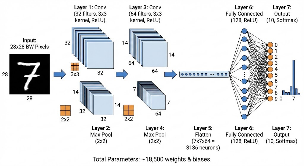
Flattening: This is where all of the arcane new concepts tie back into the traditional feed-forward neural network. Using our final matrices, our model will turn them into a 1-dimensional vector of all the matrices’ values lined up. If you pass through 3 6x6 matrices, you’ll receive a vector with 12*12*3 = 432 elements. Thus, your initial flattening layer should have 432 neurons. Later, you could have another layer with 216 neurons, and finally an output layer with as many neurons as there are output classes
Finally, we can put together a full convolutional neural network. Of course, there are many possible combinations of layers, but this is a standard CNN:
V. Conclusion
I hope this clears some aspects of the CNN architecture up. This felt more like a lecture, so I’m going to make a new post comparing the performance & efficiency of MNIST digit classification using a CNN vs. a regular, feed-forward ANN.